
|
Home
|
Math Libraries
|
JAFLE
|
Blog
|
Contact
|
|
Showcase Builder
|
Javascript Pseudo-Compiler
|
Downloads
|
Floating-Point Numbers are dead.
Floating-Point Numbers are dead!
Long live Fractional Computation!
JABigInt & JABigFraction
- Math libraries are software development tools
- JABigInt is at least 4X faster than all other integer libraries
- JABigInt facilitates encryption of live streaming video at higher resolutions
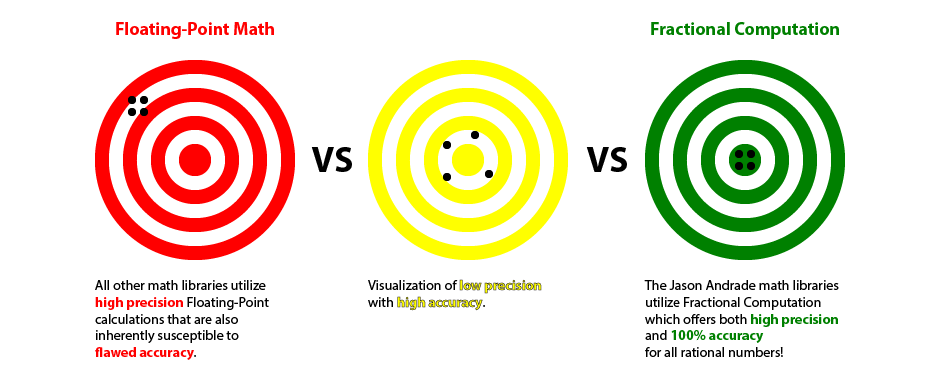
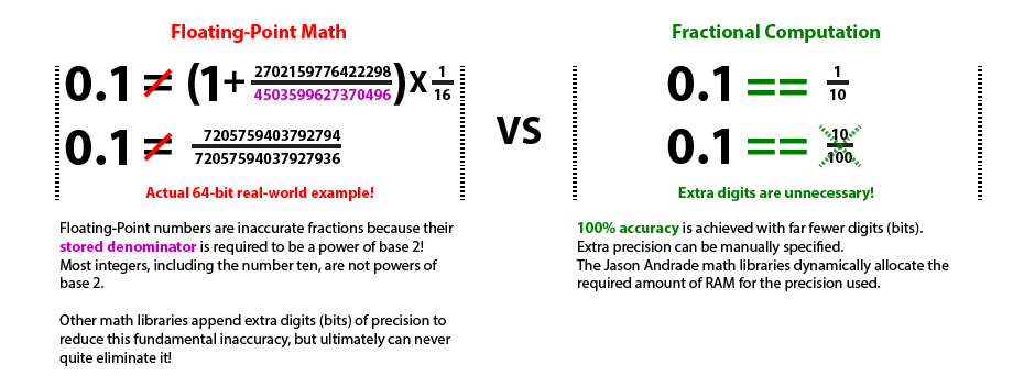
- Applications that rely on floating-point or fixed-point arithmetic are subject to rounding errors
- Fractions are inherently 100% accurate for all rational numbers
- JABigFraction is the world's first complete Fractional Computation math library
- JABigFraction eliminates the possibility of rounding errors in machine decision making
- JABigFraction by extension simplifies Quality Assurance testing and reduces software maintenance
- Robotics, Autonomous Vehicles, and Rocket Trajectories, are some of the most impacted technologies
What

At least half of these delays are fundamentally caused by floating-point rounding errors.
The fuzzy logic used to manage the inaccuracy of floating-point numbers in traditional software development is highly susceptible to environmental changes.
Leveraging Fractional Computation completely eliminates the anomalous behaviours that regularly appear when utilizing now obsolete floating-point math!
JABigInt & JABigFraction are dynamic-precision math libraries that unlock the power of Fractional Computation.
JABigInt & JABigFraction
- The only set of math libraries capable of fractional computation that
supports all Arithmetic and Trigonometric functions - Currently available 32-bit version offers
native Objective-C support for Apple's iOS platform (iPhone & iPad) - Compatible with the latest 32-bit and 64-bit Apple iDevices and iOS versions
- 64-bit and/or C/C++ versions can be created upon request for most platforms
- Contractually guaranteed to be 100% bug free
- Utilize decimal point number conversion methods to facilitate interaction with end-users
- Over 631,000 digits of precision
- Iterative Number Theoretic Transform Multiplication
is at least 8 times faster than the obsolete recursive FFT used by GMP - Are the silver bullet needed to produce the next generation of apps
in the fields of Scientific Research, Engineering, Manufacturing, and Finance
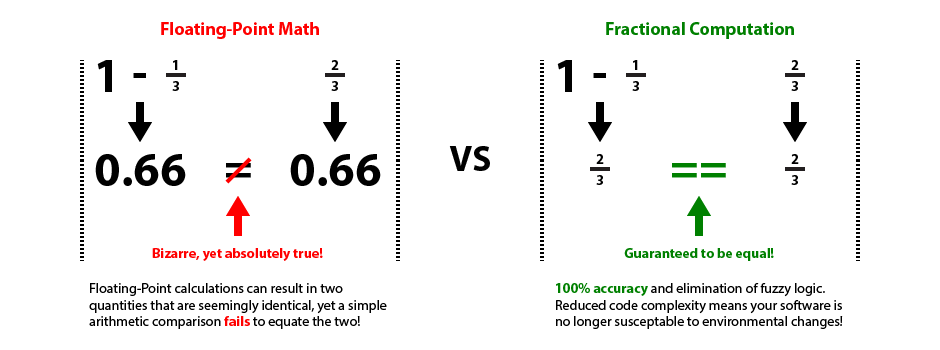
Software often makes thousands of decisions a second based on floating-point comparisons. Direct comparisons between floating-point numbers fail extremely often because of rounding errors. The term Fuzzy Logic originally referred to the extra code needed to make useful floating-point number comparisons. Fuzzy Logic introduces an extra constant when comparing two quantities, such that a floating-point number is effectively compared against a range instead of a fixed value. Fractional Computation never has rounding errors when dealing with Rational Numbers, thus eliminating the need for Fuzzy Logic in the first place. This reduces the complexity of your software and thus saves both money and time.
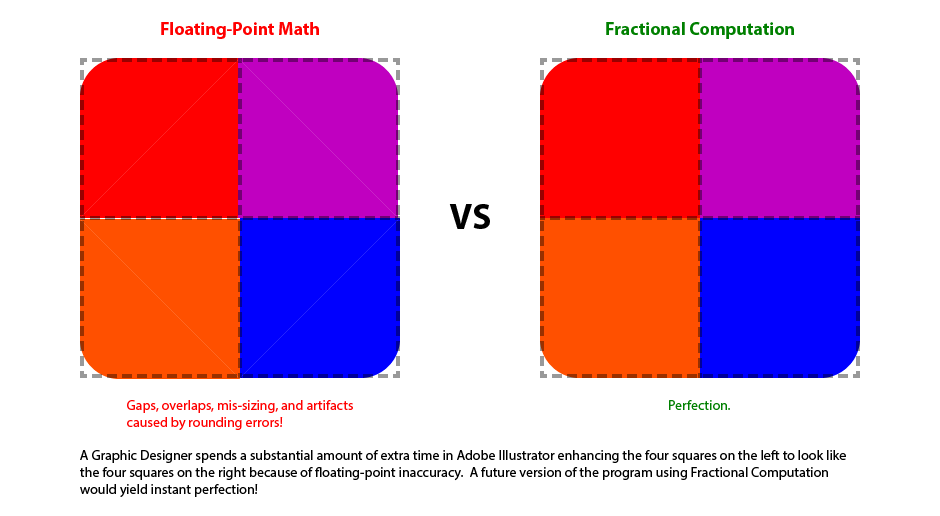
It is very difficult for your Quality Assurance department to devise test cases that anticipate all of the potential Fuzzy Logic glitches. A software module that was working months earlier might suddenly start manifesting obvious problems because the underlying cause of those bugs required very particular conditions to be met in order for them to appear. Because Fractional Computation doesn't require the implementation of Fuzzy Logic, your QA staff don't even have to attempt to deal with the related issues, thus saving both money and time.
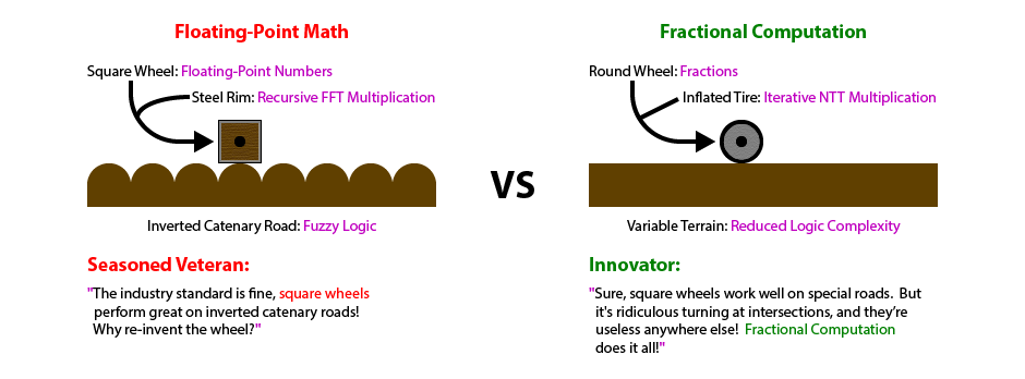
The constant used in a Fuzzy Logic comparison is tied to some real world quantity being measured (eg the size of boxes moving on a conveyor belt). If real world quantities change by an order of magnitude then the constants being used often need to be changed in numerous places within the source code. For instance, if your business either miniaturizes or jumbo sizes a product that needs to be measured while moving on a hypothetical conveyor belt. If these constants are correct in most places, yet wrong in even a single location, your software will behave fine most of the time but every so often do something "crazy". It takes an inordinate amount of time to track down and eliminate such inconsistent glitches after the fact. Fractional Computation prevents the need for this maintanence, and thus eliminates all of the associated project delays!
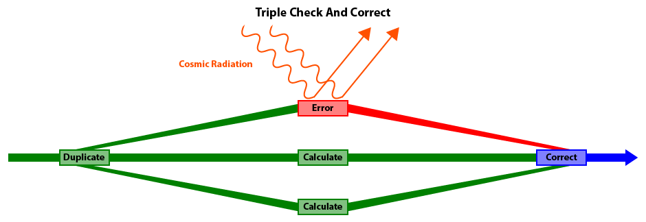
One unusual problem in the aerospace industry is the effect of cosmic radiation on integrated circuits
(computer chips).
At high altitudes and in the vacuum of space, microwaves and other forms of cosmic radiation can occasionally flip a random bit and cause a program glitch.
The Triple Check And Correct functions in the Jason Andrade Math Libraries can be used to detect and compensate for such occurances and thus improve overall reliability of a system.
When your large corporation is ready to save millions every year, contact Jason Andrade.
Why
When your large corporation is ready to save millions every year, contact Jason Andrade.
How
Once fully optimized the Iterative Number Theoretic Transform Multiplication Algorithm is the fastest way to multiply two integers larger than the size of a CPU's registers. The NTT (Number Theoretic Transform) is essentially a superior alternative to the Fast Fourier Transform algorithm because it only requires the CPU to perform integer operations. By avoiding both the floating-point operations and complex numbers required by an FFT, an iterative NTT implementation is at least 4 times faster.
Multiplication is the cornerstone operation that directly impacts the performance of most functions in any math library.
What's described here is at least 10 steps beyond any other publically accessible document.
Understand that the implementation used by the commercial Jason Andrade Math Libraries is at least four times more complex and four-fold faster than what is shown here.
Using an NTT (Number Theoretic Transform) to multiply two numbers involves the following basic execution steps:
from the time domain into the frequency domain.
and multiply the individual pairs together to generate the new convolution set.
Before we can begin to implement an NTT the size of our prime number must be chosen. We can't calculate the actual value of the prime number quite yet, just establish a fixed size. On a 32-bit computer (ie older iPhones) it is optimal to choose a prime number that's exactly 31-bits wide. This 31-bit prime number will be the divisor used in all modulus operations. In order to leverage Montgomery's Modulo Multiplication Method it's necessary to use a prime that's one bit smaller than \( \require{color} \definecolor{blue}{RGB}{0, 0, 255} \definecolor{orange}{RGB}{255, 80, 0} \definecolor{purple}{RGB}{192, 0, 192} \definecolor{red}{RGB}{255, 0, 0} sampleBitCapacity \).
They are actually used most often in Digital Signal Processing.
One example DSP function is frequency shifting.
Frequency shifting can be used to play music faster without the vocals sounding like a chipmunk.
It's vitally important to establish the distinction between the terms "samples" and "input samples".
For reasons that will become obvious in the first step of implementation, we can't simply use our raw data set as input samples!
Let's say our raw input numbers are organized as arrays of 32-bit segments.
The data segments of each raw input array will need to be further broken up into smaller input samples.
In the case of a 32-bit computing platform we'll likely end up using input samples with an \( inputSampleBitSize \) (the actual bit size of a value, excluding preceding zero bits) of either 8 bits or 4 bits.
However, during the execution of an NTT algorithm the 8-bit or 4-bit input samples will tend to expand to the size of the prime number used (31 bits).
It's therefore necessary to store these input samples in an array of unsigned integers, a data type that supports a \( sampleBitCapacity \) of 32 bits.
Thus once execution of the NTT algorithm commences the former
"input samples" are referred to as merely "samples".
If you plan on implementing a 32-bit NTT solution, simply scroll to Preparation Step #3 and use the supplied table of constants and associated 31-bit prime number.
Preparation Step #1: Calculating the safe maximum number of samples
Before we can calculate the safe maximum number of samples it's necessary to extend both input numbers with prefixed zero valued input samples such that they conform to all three of the following rules:
In order to conform to just Rule #1, two example input data sets of sizes 28 and 15
would need to be extended to at least 32 and 16 samples, respectively.
In order to conform to both Rule #1 and Rule #2, two example input data sets of sizes 28 and 15
would both need to be extended to at least 32 samples each.
must be greater than or equal to the sum of the number of samples in the unextended data sets.
In order to conform to all three Rules, two example input data sets of sizes 28 and 15
would both need to be extended to at least 64 samples each because \( \textcolor{blue}{\textbf{(}} 28 \textcolor{red}{\boldsymbol{+}} 15 \textcolor{blue}{\textbf{)}} \textcolor{orange}{\boldsymbol{>}} 32 \).
Exceeding the safe sample quantity limit can potentially cause an overflow and generate an erroneous result.
The safe maximum number of samples is a power of base 2 that is calculated as a function of the bit size of the prime number used and the maximum bit size of the individual input data samples.
The bit size of a number is the quantity of digits in the binary representation of that number, excluding all preceding zeros.
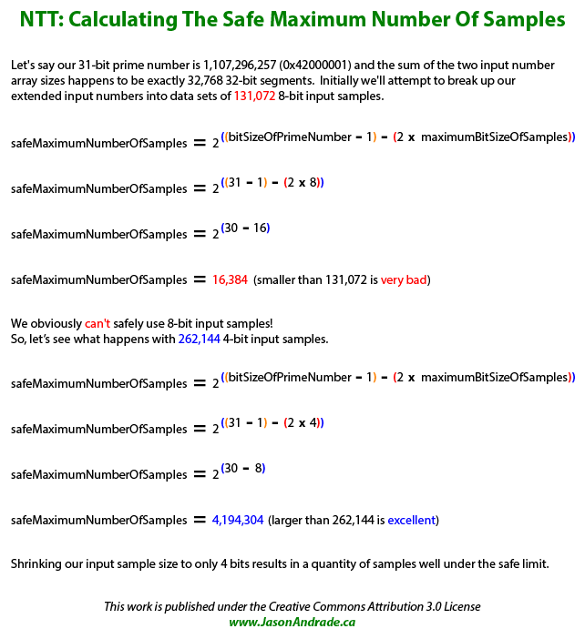
Based on this equation, software may only use 8-bit samples with input numbers that have been extended to no larger than 4,096 32-bit segments. All input numbers bigger than this must use 4-bit samples instead, but are constrained to an extended size that is smaller than the absolute limit of 524,288 32-bit segments. Using 8-bit samples whenever possible considerably reduces the number of calculations that need to be performed and is thus advantageous. Don't reduce the input sample size to less than 4 bits because doing so will cause problems in Execution Step #5.
In instances where the input sample size cannot be reduced it will be necessary to choose a larger prime number and implement buffer arrays whose data type is bigger than a 32-bit Unsigned Int.
Use the following reconfigured equation to determine the minimum bit-size of a suitable prime number:
$$ minimumBitSizeOfPrimeNumber \textcolor{orange}{\textbf{ = }} \textcolor{blue}{\textbf{Log}} \textcolor{blue}{\boldsymbol{_2}} \textcolor{blue}{\textbf{(}} numberOfSamples \textcolor{blue}{\textbf{)}} \textcolor{red}{\boldsymbol{+}} \textcolor{purple}{\textbf{(}} \textcolor{blue}{\textbf{2}} \textcolor{red}{\boldsymbol{ \times }} maximumBitSizeOfSamples \textcolor{purple}{\textbf{)}} \textcolor{red}{\boldsymbol{+}} \textcolor{blue}{\textbf{1}} $$
Preparation Step #2: Finding and hard-coding a viable prime number and its associated \( primaryL \)
Finding a viable prime number is actually quite tricky because we also need to simultaneously find a second value called L! This L constant we are finding is actually more appropriately referred to as \( primaryL \) because it's only valid for a theoretical sample set containing a single element. In reality NTT Multiplication requires actual sample sets that consist of at least 2 elements in order to work. Furthermore, if the input numbers are small enough that they can be stored in CPU registers then it will always be more efficient to multiply them in hardware.
There are three rules that severely restrict viable values for both the prime number and the \( primaryL \) constant:
The following methodology is adequate to calculate these values under most circumstances.
First, generate a set of probable prime number candidates.
The first candidate should only have two 1 bits, with all other bits set to zero.
Since we need a 31-bit prime number, the 31st least significant bit (counting from the right) is set to 1.
The least significant bit is also set to 1 in order to guarantee an odd number (all prime numbers are odd).
The other twenty-nine potential candidates each have exactly three 1 bits.
They are permutations of the first candidate and are generated by individually flipping each of the twenty-nine 0 bits between the two original 1 bits.
Now we need to confirm that these potential candidates are in fact prime numbers! The easiest way to do this is to simply utilize one of the myriad prime number reference websites, like NumberEmpire.com. This reduces our list of 30 potentials down to only 8 prime number candidates.
Since \( primeNumber \) and \( primaryL \) are both frequently used constants during the execution of the NTT algorithm, it makes a whole lot more sense to pre-calculate them instead of trying to find them at run-time. That said, it's necessary to write a small brute force program (FindPrimaryL) to determine which of our candidate primes is suitable and its corresponding \( primaryL \) constant.
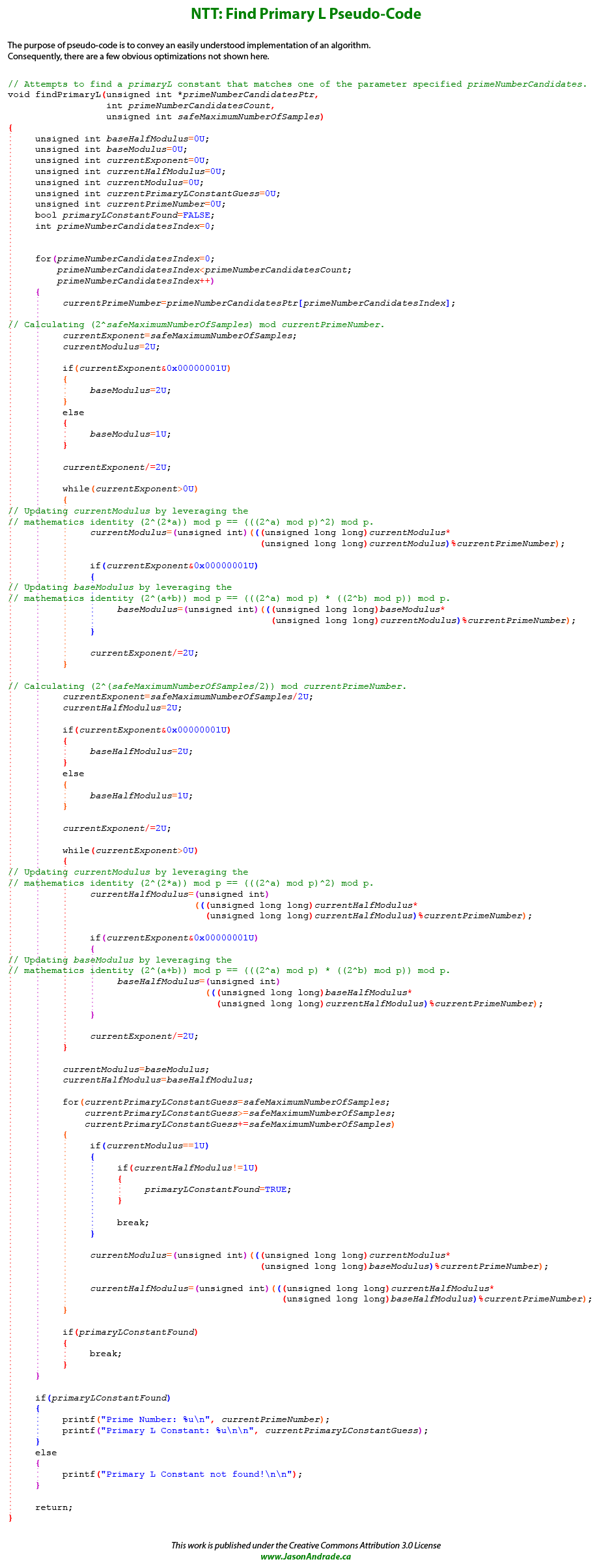
Out of the eight 31-bit prime number candidates, FindPrimaryL happens to identify the last one as suitable for our present purposes. From this point forward \( primeNumber \) is 1,107,296,257 (Hexadecimal: 0x42000001), with a \( primaryL \) constant of 50,331,648 (Hexadecimal: 0x3000000).
If you are implementing a different solution (for example, 63-bit), FindPrimaryL might fail to identify an acceptable prime number. In which case it will be necessary to generate some additional potential prime number candidates, this time exploring permutations with four 1 bits.
Preparation Step #3: Precalculate the table of constants for every valid quantity of samples
For every valid quantity of samples in a subset, several constants must be calculated. It is in fact ideal to hard code these values into arrays instead of calculating them at run-time. Normally NTT Multiplication involves just the \( WConstant \), \( inverseWConstant \), and \( reciprocalConstant \) values, but application of Montgomery's Modulo Multiplication Method necessitates the usage of left-shifted modulii as well. We will once more need to write another small program (calculateExponentiatedModulus) that leverages the following two math identities to calculate these values:
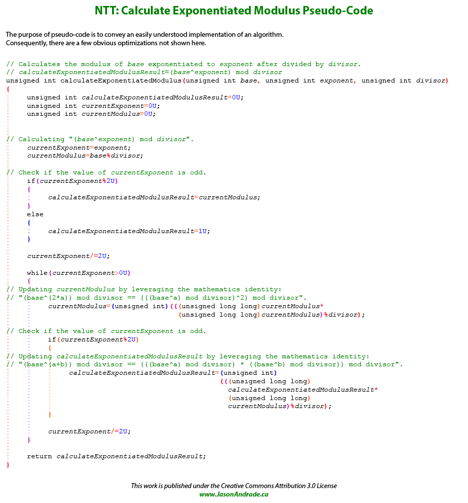
Valid \( numberOfSamples \) values are all powers of base 2 ranging from 2 to \( safeMaximumNumberOfSamples \).
Each of the following constants must now be pre-calculated for every valid \( numberOfSamples \):
Preparation Step #4: Using Montgomery's Modulo Multiplication Method
Montgomery's Modulo Multiplication Method (MMMM) is a means of calculating the modulus of a product without performing a division operation. Division is notoriously computation intensive, even when implemented at the hardware level. MMMM solves the following equation using three multiplications, one subtraction, plus sometimes an extra addition: $$ finalModulus \textcolor{orange}{\textbf{ = }} \textcolor{blue}{\textbf{(}} firstFactor \textcolor{red}{\boldsymbol{ \times }} secondFactor \textcolor{blue}{\textbf{)}} \textcolor{red}{\textbf{ mod }} primeNumber $$
Additional requirements based on a 32-bit implementation:
a 32-bit implementation cannot utilize a prime number larger than 31 bits.
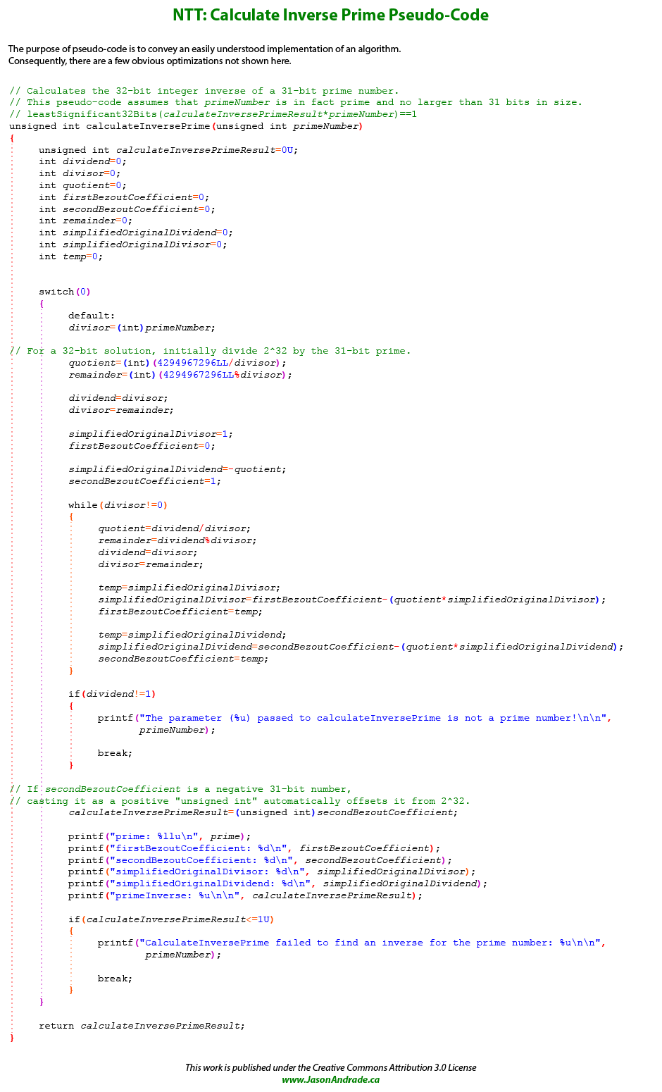
It is also necessary to pre-calculate two more values, the integer inverse of \( primeNumber \), and the left-shifted modulus of \( secondFactor \).
Finding the integer inverse of our prime number is most efficiently achieved by utilizing Bézout's extension of the Euclidean Algorithm. Please note that the "Method Of Least Absolute Remainders" enhancement of Euclid's basic algorithm isn't compatible with Bézout's extension. The \( inversePrime \) is essentially a 32-bit or smaller number that when multiplied with our prime number will generate a product whose least significant 32 bits has a value of one.
For a 32-bit solution the initial dividend is set to \( 2^{32} \) (4,294,967,296), and the initial divisor is set to \( primeNumber \) (1,073,741,827). Just like the basic Euclidean Algorithm, execution ends once an iteration yields a remainder of zero. Once the algorithm finishes, if \( secondBezoutCoefficient \) is a positive number then that is our \( inversePrime \). Otherwise, \( inversePrime \) is determined by adding \( secondBezoutCoefficient \) to \( 2^{32} \) (4,294,967,296). Yet again, another small program (calculateInversePrime) needs to be written. It determines that this particular \( inversePrime \) is calculated to be 3,187,671,041 (Hexadecimal: 0xBE000001). A more detailed description of the Extended Euclidean Algorithm is presented in the Fraction Simplification section of this page.
Precalculating \( secondFactorLeftShiftedModulus \) is as easy as it sounds.
Simply bitwise left-shift \( secondFactor \) by 32 bits and then divide by \( primeNumber \) to obtain the modulus (remainder).
This left-shift is analogous to multiplying \( secondFactor \) by \( 2^{32} \).
The following math identity shows how adding 32 to the exponent of a power of base 2 is equivalent to multiplying that power by \( 2^{32} \), even when performing modulo arithmetic:
$$ \textcolor{purple}{\textbf{(}} 2^{ \textcolor{blue}{\textbf{(}} a \textcolor{red}{\boldsymbol{+}} 32 \textcolor{blue}{\textbf{)}} } \textcolor{purple}{\textbf{)}} \textcolor{red}{\textbf{ mod }} divisor \textcolor{orange}{\textbf{ = }} \textcolor{purple}{\textbf{(}} \textcolor{blue}{\textbf{(}} \textcolor{red}{\textbf{(}} 2^a \textcolor{red}{\textbf{)}} \textcolor{red}{\textbf{ mod }} divisor \textcolor{blue}{\textbf{)}} \textcolor{red}{\boldsymbol{ \times }} \textcolor{blue}{\textbf{(}} \textcolor{red}{\textbf{(}} 2^{32} \textcolor{red}{\textbf{)}} \textcolor{red}{\textbf{ mod }} divisor \textcolor{blue}{\textbf{)}} \textcolor{purple}{\textbf{)}} \textcolor{red}{\textbf{ mod }} divisor $$
Within the context of NTT Multiplication most of the constants we've pre-calculated will become the \( secondFactor \) whenever MMMM is used. The equations for the left-shifted modulii variants calculated in Preparation Step #3 are thus derived by adding 32 to the exponents of the equations used to compute the associated normal constants.
MMMM is obviously only efficient when it's necessary to calculate \( finalModulus \) for multiple values of \( firstFactor \), but with both the \( secondFactor \) and \( primeNumber \) always remaining unchanged.
David Harvey has reported a performance improvement of over 50% when compared with a plain NTT implementation.
Comparison Of NTT Implementations
A Number Theoretic Transform is typically described as a recursive algorithm because that version is easier to comprehend. However, it's the iterative version that's faster in a real-world implementation!
All NTT implementations process an input sample set multiple times, in what are referred to as layers.
In a recursive implementation an input sample set is broken up into subsets, with each layer adjusting both the number of subsets and the quantity of samples in each subset.
Each layer of a recursive NTT implementation splits its samples into even and odd relatively indexed subsets and performs a recursive function call on each subset independently.
The current layer is only processed after these recursive calls have completed execution.
If a sample set has only two elements then no recursive calls occur and it is simply processed and returns execution to the previous layer.
Effectively we're repeatedly dividing the input sample set into two until we end up with a bunch of subsets containing exactly two samples.
These subsets are first processed and then the previous layer processes the joined output sample sets that become twice as large.
A recursive NTT implementation ultimately collapses back to the original sample set (with updated values) after it has been processed.
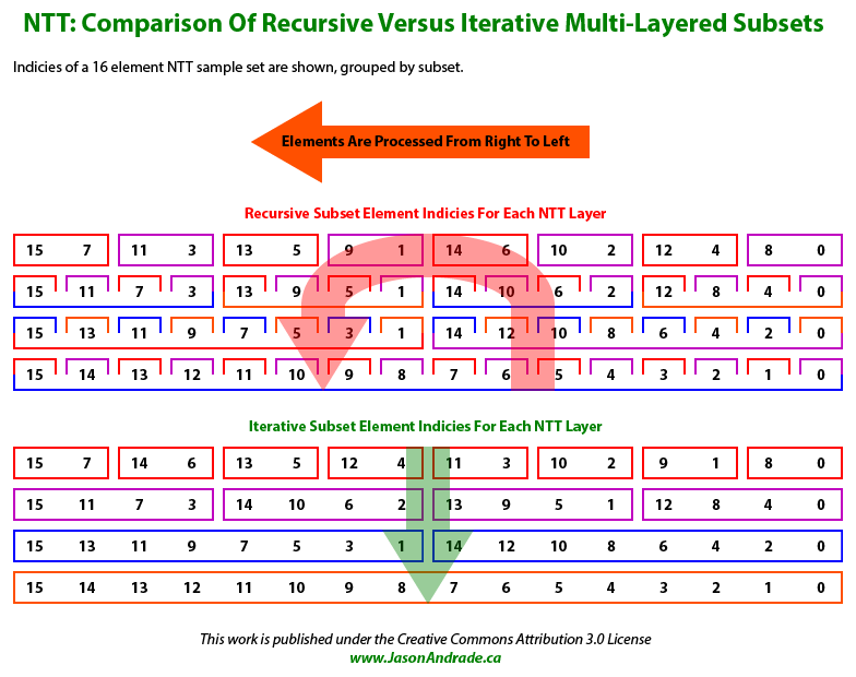
An iterative solution on the other hand simply starts with many subsets consisting of pairs of samples and repeatedly combines them.
The iterative methodology allows for subsets to be processed by sequential indices, thus facilitating optimizations that can't be utilized by a recursive solution.
In addition, a recursive implementation requires the creation of a separate additional buffer for each layer of the transform.
Because an iterative implementation only requires a single extra buffer it has a much smaller memory (RAM) footprint.
Furthermore, while a recursive implementation requires the use of copy operations while assembling subsets,
an iterative solution avoids this performance penalty by directly accessing the elements within a subset.
This is done to facilitate hardware accelerated vector computing (ARM NEON Intrinsics), also known as SIMD, SIMT, or on-chip parallel processing.
Utilization of vector computing results in an over 80% increase in performance on an ARMv7 CPU, which translates to a roughly 45% reduction in execution time.
Iterative Number Theoretic Transform Implementation
Prior to processing an extended input sample set with the NTT it's vitally important to reverse the order of the samples, so that the most significant sample is stored at index zero in the array. Please note that this reversal of the sample ordering occurs after the input sample sets are extended with prefixed zero valued input samples according to the three rules mentioned in Preparation Step #1.
The first (outermost) loop is responsible for stepping through each layer of the transform. It is implemented with exactly \( \textcolor{blue}{\textbf{Log}} \textcolor{blue}{\boldsymbol{_2}} \textcolor{blue}{\textbf{(}} numberOfSamples \textcolor{blue}{\textbf{)}} \) iterations.
This first loop keeps track of \( numberOfSubsetsInLayer \), which is initialized to \( sampleSetHalfSize \)
(half the number of input samples) and repeatedly halves in value per iteration.
The loop continues to iterate while \( numberOfSubsetsInLayer \) is greater than zero.
The \( numberOfSamplesPerSubset \) variable is initialized to 2 for the first layer of the transform and doubles in value for each successive layer.
Each layer of the NTT utilizes values from the precalculated constants table generated in Preparation Step #3.
The row of constants used for a particular NTT layer is keyed to the \( numberOfSamples \) field in the table being equal to \( numberOfSamplesPerSubset \).
The processing of sample pairs within the third (innermost) loop requires exponentiating the \( WConstant \) referenced from this row in the table.
The exponent increments by one for each successive pair of samples within each subset being processed.
Since every subset within an NTT layer always contains exactly the same number of samples, the exact same powers of \( WConstant \) are used to process each subset.
It's therefore most efficient to calculate these powers of \( WConstant \) (using MMMM) within the outermost loop, but prior to the second (middle) loop, and store them in an array.
More accurately it's the left-shifted modulus of these powers that's stored in the array since they are exclusively used as \( secondFactor \) in subsequent MMMM operations.
Henceforth these left-shifted modulii of the \( WConstant \) powers shall be referred to as the subset constants array and indexed by \( currentSubsetConstantIndex \).
The value of \( currentSubsetConstantIndex \) is always equal to the exponent used to generate the value stored in the array at that same index.
The number of subset constants calculated and stored in the array is always equal to half of \( numberOfSamplesPerSubset \).
The first subset constant (at index zero) is always equal to the left-shifted modulus of \( WConstant^0 \) (one), which for our 31-bit \( primeNumber \) (1,107,296,257)
is always equal to 973,078,525.
The second subset constant (at index one) is always equal to the \( WConstantLeftShiftedModulus \) that's directly referenced from the precalculated constants table generated in Preparation Step #3.
The second (middle) loop increments through each subset within the current NTT layer (as defined by the first loop). The loop counter, \( currentSubsetIndex \), is initialized to zero and increments by one for \( numberOfSubsetsInLayer \) iterations. Samples within the current subset (as defined by the second loop) are processed in non-sequentially indexed pairs. Furthermore, the Even/Odd sample pairs read from the previous layer generate a pair of Addition/Subtraction samples that are written to non-matching indices in the current layer.
The third (inner) loop keeps track of both the index of the previous layer's Even sample being processed as well as the index of the current layer's Addition sample being generated.
Generation of the current NTT layer actually occurs within this third loop.
Both \( previousLayerEvenSampleIndex \) and \( currentLayerAdditionSampleIndex \) are initialized to \( currentSubsetIndex \).
However, while \( previousLayerEvenSampleIndex \) increments by double \( numberOfSubsetsInLayer \), \( currentLayerAdditionSampleIndex \) increments by only \( numberOfSubsetsInLayer \).
The loop persists only while \( currentLayerAdditionSampleIndex \) is less than the sum of \( currentSubsetIndex \) and \( sampleSetHalfSize \).
The index of the Odd sample to be read from the previous layer is equal to the sum of \( previousLayerEvenSampleIndex \) and \( numberOfSubsetsInLayer \). The index of the Subtraction sample to be written to the current layer is equal to the sum of \( currentLayerAdditionSampleIndex \) and \( sampleSetHalfSize \).
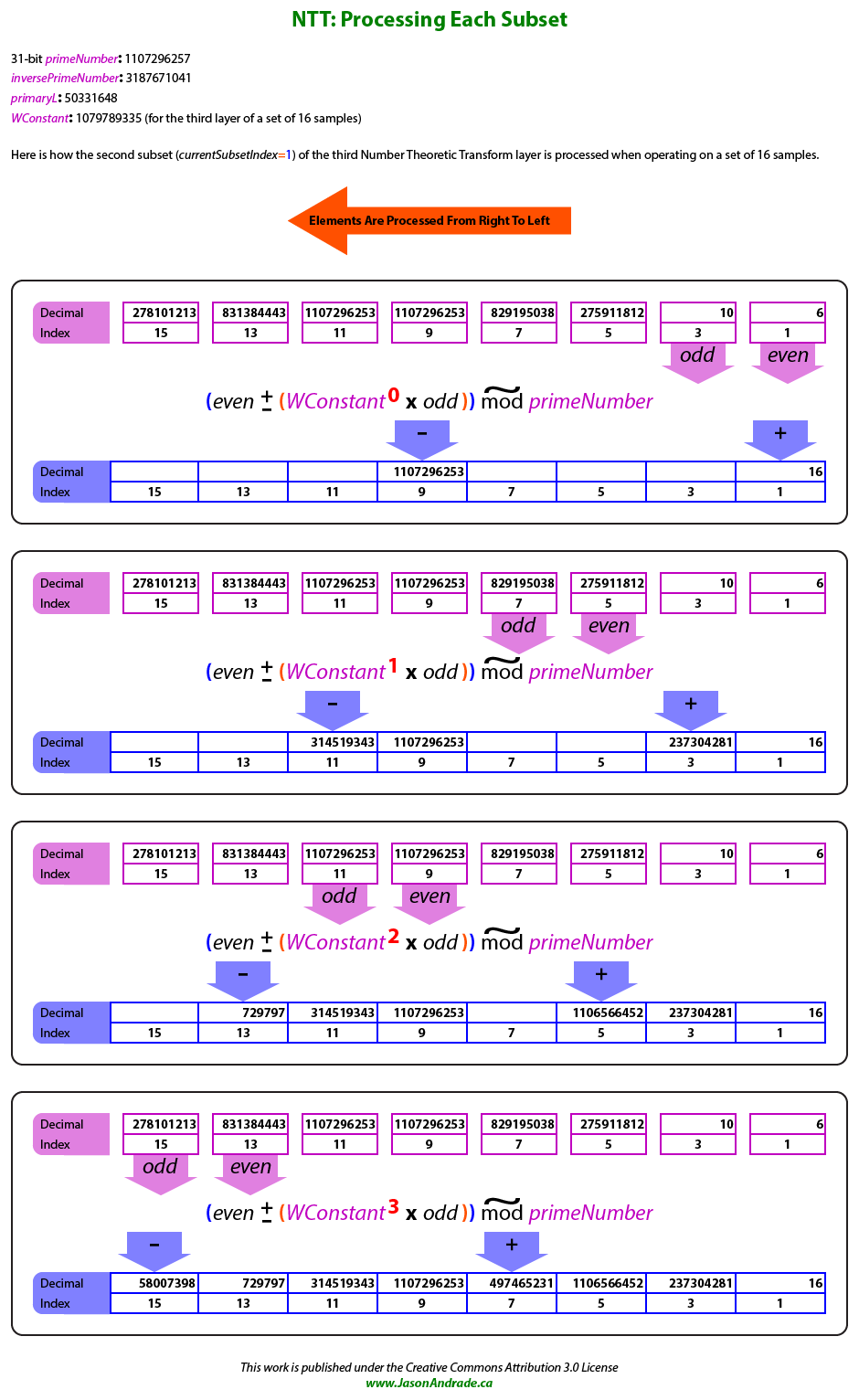
The following expression is used to generate the Addition/Subtraction samples:
$$ \textcolor{purple}{\textbf{(}} even \textcolor{red}{\boldsymbol{\pm}} \textcolor{blue}{\textbf{(}} WConstant^{currentSubsetConstantIndex} \textcolor{red}{\boldsymbol{ \times }} odd \textcolor{blue}{\textbf{)}} \textcolor{purple}{\textbf{)}} \ \textcolor{red}{\boldsymbol{\widetilde{mod}}} \ primeNumber $$
This expression expands to:
$$ \textcolor{purple}{\textbf{(}} even \textcolor{red}{\boldsymbol{\pm}} \textcolor{orange}{\textbf{(}} \textcolor{blue}{\textbf{(}} WConstant^{currentSubsetConstantIndex} \textcolor{red}{\textbf{ mod }} primeNumber \textcolor{blue}{\textbf{)}} \textcolor{red}{\boldsymbol{ \times }} odd \textcolor{orange}{\textbf{)}} \textcolor{red}{\textbf{ mod }} primeNumber \textcolor{purple}{\textbf{)}} \ \textcolor{red}{\boldsymbol{\widetilde{mod}}} \ primeNumber $$
As shown in the expansion of the expression, two regular \( \textcolor{red}{\textbf{mod}} \) operations and one unusual \( \textcolor{red}{\boldsymbol{\widetilde{mod}}} \) operation are actually used.
For Addition samples, the \( \textcolor{red}{\boldsymbol{\widetilde{mod}}} \) operation doesn't utilize division, instead \( primeNumber \) is subtracted from the intermediate value if it is greater than \( primeNumber \).
In the case of Subtraction samples, \( primeNumber \) is added to them if their intermediate value is less than zero.
The following illustration shows an example excerpt of the larger run-through presented farther down this page.
This excerpt describes in greater detail the sample generation of the
second subset (\( currentSubsetIndex \textcolor{orange}{\textbf{ = }} \textcolor{blue}{\textbf{1}} \)) for the third NTT layer of \( firstFactor \).
NTT Multiplication Execution
If either of the two factors being multiplied is zero, then simply return a zero result.
If either of the two factors being multiplied is equal to positive one, then simply return the other factor as the result.
If either of the two factors being multiplied is equal to negative one, then simply return the additive inverse of the other factor as the result.
If both of the two factors being multiplied are 32 bits or less then their absolute values can be cast as 64-bit unsigned integers and multiplied natively in hardware, with the sign of the product calculated separately.
32-bit CPUs are in fact capable of multiplying two 32-bit registers and storing the resulting product in a combined 64-bit register (yes, they all have one).
Execution Step #1: Break up each of the two input numbers into factor sets of smaller data samples
The sign of the product is determined in advance to be negative if only one of the two factors is a negative number, otherwise it will be positive.
The signs of both input numbers are stripped, ensuring that they are both positive integers.
Break up, extend, and store the two factors being multiplied into two unsigned integer (32-bit) arrays in accordance with the requirements outlined in Preparation Step #1.
8-bit samples can be used if doing so results in fewer than 16,384 samples in an extended input sample set.
This effectively means that the larger and more efficient 8-bit samples can be used if the sum of the bit sizes of the two factors being multiplied is less than or equal to 131,072 bits.
More than this requires that 4-bit samples be used.
If the sum of the bit sizes of the two factors being multiplied is greater than 16,777,216 bits (4,194,304 4-bit samples),
then a 32-bit (31-bit prime number) NTT simply cannot be performed.
Don't forget to store the individual input samples into their respective arrays in reverse order, such that the most significant sample for each input number is stored at index zero in its respective array.
Execution Step #2:
Use an NTT to individually translate each factor set of data samples from the time domain into the frequency domain
Both of the two input sample sets need to be separately processed by the NTT.
A naive implementation would finish processing all NTT layers on the first factor set before processing the second factor.
However, it's possible to process each layer of the NTT on both sample sets consecutively before proceeding to the next layer.
This allows us to reuse the same subset constants for both sample sets without having to wastefully recalculate them.
In addition to each of the active buffers used by the two sample sets awaiting processing, a separate third buffer is needed to store the generated samples of the current layer.
Because we're only actually processing one sample set at a time, it's most efficient to implement a triple buffer system with a rotating empty buffer.
Once a sample set is processed, the formerly active buffer becomes the new empty buffer.
Execution Step #3:
Pair up the samples between the two factor sets and multiply the individual pairs together to generate the new convolution set
Each pair of samples read from the same indices across both entire active sample set arrays are multiplied together, with each product divided by \( primeNumber \) and the resulting modulii stored in a newly generated convolution sample set array.
Execution Step #4: Apply the inverse NTT to the convolution set
The inverse NTT is only applied to the single convolution sample set and has a few differences from the NTT algorithm already described. When applying the inverse NTT to the convolution sample set the order of the samples is not initially reversed. The constants table created in Preparation Step #3 defines the \( inverseWConstant \) and \( inverseWConstantLeftShiftedModulus \) values to be used instead of the \( WConstant \) and \( WConstantLeftShiftedModulus \) values. The final step in applying the inverse NTT requires that the samples in the convolution sample set be reciprocated. Rectify the sample set by multiplying each sample by the \( reciprocalConstant \) keyed to \( numberOfSamples \) and storing the modulus after dividing the resulting product by \( primeNumber \). This is in fact best accomplished by leveraging MMMM with \( reciprocalConstantLeftShiftedModulus \) as described in Preparation Step #4.
Execution Step #5: Trim and realign the now rectified convolution set
An unfortunate side effect of NTT Multiplication is the concatenation of extra zero samples to one or both ends of the sample set. All least significant samples (counting upwards from index 0) with a value of zero can immediately and unconditionally be trimmed. The exact number of most significant samples that need to be trimmed is more difficult to determine because some zero samples might be needed to generate the correct final result. We know with absolute certainty that the maximum bit size of the correct final result is equal to the sum of the bit sizes of the two factors being multiplied. The minimum bit size is also guaranteed to be one less than the maximum. In Execution Step #6 the 32-bit samples will be recombined with staggered addition, whose potential carry bit introduces another bit of uncertainty. This means that a valid bit-size for a projected correct final result lies within a three bit range. Since each sample trimmed reduces the bit-size of the final result by 4 or 8 bits (determined by the \( inputSampleBitSize \) chosen at the very beginning of the implementation) it's possible to correctly predict how many most significant samples should be trimmed.
The number of samples trimmed thus far is deducted from \( sampleSetSize \) to calculate \( adjustedSampleSetSize \). Now divide \( sampleBitCapacity \) by \( inputSampleBitSize \) to determine how many least significant samples need to be analyzed to determine \( leastSignificantSamplesCount \). During analysis the least significant (after initial trimming) convolution sample is associated with a \( sampleBitSizeOffset \) of zero. Increment \( sampleBitSizeOffset \) by \( inputSampleBitSize \) for each successive convolution sample being analyzed. For each sample, the \( sampleBitSizeDifferential \) is calculated by subtracting \( sampleBitSizeOffset \) from the sample's bit-size. The \( leastSignificantSampleEffectiveBitSize \) is then set to the largest \( sampleBitSizeDifferential \) of all the samples being analyzed. $$ minimumProductBitSize \textcolor{orange}{\textbf{ = }} leastSignificantSampleEffectiveBitSize \textcolor{red}{\boldsymbol{+}} \textcolor{blue}{\textbf{(}} \textcolor{purple}{\textbf{(}} adjustedSampleSetSize \textcolor{red}{\boldsymbol{-}} \textcolor{blue}{\textbf{1}} \textcolor{purple}{\textbf{)}} \textcolor{red}{\boldsymbol{ \times }} inputSampleBitSize \textcolor{blue}{\textbf{)}} $$ If \( minimumProductBitSize \) is greater than \( maximumProductBitSize \) then it becomes necessary to trim the most significant samples (counting downwards from index \( adjustedSampleSetSize \textcolor{red}{\boldsymbol{-}} \textcolor{blue}{\textbf{1}} \)). $$ extraProductBitsCount \textcolor{orange}{\textbf{ = }} minimumProductBitSize \textcolor{red}{\boldsymbol{-}} maximumProductBitSize $$ $$ mostSignificantSamplesMaximumTrimCount \textcolor{orange}{\textbf{ = }} \textcolor{red}{\textbf{RoundUp}} \textcolor{blue}{\boldsymbol{\bigg(}} \frac{extraProductBitsCount}{inputSampleBitSize} \textcolor{blue}{\boldsymbol{\bigg)}} $$ Only trim up to \( mostSignificantSamplesMaximumTrimCount \) samples that contiguously have a value of zero. Update \( adjustedSampleSetSize \) accordingly.
Execution Step #6: Recombine the samples of the rectified convolution set to generate the final result
During recombination samples are process from the most significant (highest index)
to the least significant (lowest index).
The samples are summed together, but with each successive sample bitwise left-shifted by an additional \( inputSampleBitSize \) relative to the sample preceding it.
Apply the sign precalculated in Execution Step #1 to this sum to determine the final product of the two input factors being multiplied.
High Resolution NTT Multiplication Run-Through Illustration

High Resolution NTT Multiplication Run-Through Illustration
Iterative NTT Multiplication Pseudo-Code

Iterative NTT Multiplication Pseudo-Code
When dividing a dividend bigger than the largest register on a computer's CPU, the arithmetic approach to the problem is outperformed hands-down in most cases by a binary logic solution.
This is because Mathematicians,
as human beings, think about the problem in base 10, while the computers that actually perform the calculation operate in base 2!
When viewed from the perspective of a computer, Shifted Subtraction has two main advantages over arithmetic solutions that are derived from Newton's Method.
Both the binary logic solution and an arithmetic approach to division essentially start with a gross approximation for the quotient and use an iterative process that refines down to the correct result.
However, only Shifted Subtraction can detect in advance if the correction of an iteration will overshoot the final answer before it is even applied.
Furthermore, in the case of
Shifted Subtraction each correction is calculated using relatively simple "bit shift" and "bitwise OR" operations.
Arithmetic solutions on the other hand always perform a CPU intensive calculation for every iteration and thus inefficiently compensate for overshoots with future iterations.
It is reasonable to assert that the average density of one-bits within the quotients of all possible division operations is 50%.
When simulating various sized quotients composed of alternating one and zero bits,
Shifted Subtraction yields consistently faster computation times.
The only time an arithmetic approach can outperform Shifted Subtraction is if a given quotient has a density of one-bits substantially greater than 50%.
Since it is impossible to determine the density of one-bits within a quotient before the division operation is performed, the most reasonable solution to the problem is to use Shifted Subtraction every time and understand that the average execution time in the aggregate is as low as possible.
From the binary logic perspective the bit-size of the \( quotient \) is at least the difference in bit-size between the \( dividend \) and \( divisor \), and at most one bit larger. Shifted Subtraction is an iterative algorithm that sequentially resolves the one-bits of the \( quotient \), starting with the most significant (left-most) bit. Statistically this means that the number of iterations on average is half the number of bits in the \( quotient \).
The algorithm works as follows:
Euclidean Division enhanced with the "Method Of Least Absolute Remainders" is the fastest algorithm for calculating the GCD of two integers.
The algorithm works as follows:
otherwise \( divisor \textcolor{orange}{\textbf{ = }} remainder \).
Technically the algorithm also works if we throw away both the \( dividend \) and \( divisor \) of each iteration and simply divide the \( currentRemainder \) by the \( alternateDivisor \) (or vice-versa, depending on which is larger).
At first glance this variant would seem to be beneficial because it would guarantee a smaller \( quotient \) for each division operation.
Since the speed of the division operation is determined by the size of the \( quotient \) it initially appears that this would result in a faster GCD calculation overall.
However, upon further analysis it becomes evident that the division operation can only be sped up by a single iteration at most since this variant methodology can never reduce the value of the \( quotient \) by more than half.
The original methodology presented here in depth allows for an optimization (not shown in the pseudo-code below) that checks if \( alternateDivisor \) will be smaller than \( remainder \) before it is even calculated, thus eliminating a subtraction operation for most iterations.
This pre-emptive check is performed by comparing the segment sizes of \( remainder \) and \( divisor \).
On average more processing time is saved by eliminating this subtraction operation for most GCD iterations than by eliminating a single iteration of the algorithm, and its associated division operation, for only some combinations of input numbers.
The most common method of simplifying a fraction is to divide both the \( numerator \) and \( denominator \) by the GCD of those two numbers.
However, Bézout's extension of the Euclidean Algorithm is typically around twice as fast and thus on average reduces the overall compute time by around 50%.
Please note that the "Method Of Least Absolute Remainders" enhancement of Euclid's basic algorithm isn't compatible with
Bézout's extension.
The \( numerator \) and \( denominator \) are compared (both must be integers greater than zero), resulting in the \( dividend \) and \( divisor \) being initialized to the larger and smaller of the two values, respectively.
It's important to keep track of which number was larger.
An initial division is performed to calculate the initial \( quotient \) and \( remainder \).
Initialize \( simplifiedOriginalDivisor \) to a value of one and
\( firstBezoutCoefficient \) to a value of zero.
Initialize \( simplifiedOriginalDividend \) to the additive inverse of the initial \( quotient \) and \( secondBezoutCoefficient \) to a value of one.
We now set \( dividend \) to equal \( divisor \), and \( divisor \) to equal the initial \( remainder \).
The following steps are now performed:
If the original \( numerator \) was larger than the \( denominator \) then the simplified \( numerator \) is \( simplifiedOriginalDividend \), otherwise it's \( simplifiedOriginalDivisor \). The simplified \( denominator \) is the other variable.
High Resolution Simplify Fraction Run-Through Illustration
High Resolution Simplify Fraction Run-Through Illustration
|
Home
|
Math Libraries
|
JAFLE
|
Blog
|
Contact
|
Showcase Builder
|
Javascript Pseudo-Compiler
|
Downloads
|
www.JasonAndrade.ca